

Why Observe LPV's?
What is the value of observing long-period variables (LPVs), especially visually, and continuing to do so? Let me illustrate by listing the various work that my students and I have done with your observations. Most of our results are published in JAAVSO, and some in PASP (Publications of the Astronomical Society of the Pacific). Also be sure to read the review articles by Kiss and Percy (2012 JAAVSO 40, 528) and by Willson and Marengo (2012 JAAVSO 40, 516) in the JAAVSO Centennial Issue, and check out the “LPVs in the News” web page. In my case, your observations have had educational as well as scientific value, by enabling my students to develop and integrate their science, math, and computing skills, motivated by doing real science, with real data – your data.
- An astrophysical mystery: why do a third of LPVs have a long secondary period (LSP)? Our work has discovered or refined LSPs in over a hundred LPVs (arxiv.org/abs/1607.06482, 2013 JAAVSO 41, 1; 41, 15) and provided new information which may help to solve the mystery.
- Another astrophysical mystery: why do the pulsation and LSP amplitudes in almost all LPV giants (2013 JAAVSO 41, 193) and supergiants (2014 JAAVSO 42, 1) increase and decrease by factors of 2 to 10 on time scales of about 20 pulsation periods or LSPs?
- Watching LPVs evolve: a century of your observations enables us to measure the slow period changes caused by the LPV's evolution (1999 PASP 111, 98; see also Tomas Karlsson's excellent recent work: 2014 JAAVSO 42, 280). The accuracy of this work increases as the square of the length of time of observation, so keep up the good work!
- A few LPVs vary more rapidly in pulsation period, and are probably undergoing a nuclear event called a “thermal pulse”. Your observations can help us to observe and understand the thermal pulse phenomenon (Templeton et al. 2005 Astron J 130, 776).
- Another astrophysical mystery: why are there random cycle-to-cycle period fluctuations in almost all LPVs (1999 PASP 111, 94)? Are they due to the effect of giant convection cells?
- What about the “semi-regular” (SR) LPVs? Many of them turn out to have two pulsation periods, and two periods are even better than one (2013 JAAVSO 41, 1; 41, 15)! They provide a tool for “precision astrophysics” using the Petersen diagram, a plot of period ratio versus period (2015 JAAVSO 43, 118).
- And what about all the “irregular” (L-type) LPVs in the AAVSO database? Most of them turn out to be non-variable, or micro-variable at best. In my humble opinion, they should be dropped from the program, though not everyone agrees with me (2009 JAAVSO 37, 71; 2010 JAAVSO 38, 161; 2011 JAAVSO 39, 1).
- Your observations also help us to identify LPVs with unique or peculiar behavior, which makes them worthy of more intensive study (1990 ASP CS 11, 446).
- And your observations enable us to determine reliable periods and amplitudes for hundreds of LPVs, providing raw material for many areas of astronomy and astrophysics: describing and classifying, comparing with observations at other wavelengths, scheduling observing runs, theoretical modelling of evolution, pulsation, and mass loss, and much more
This summer, my student Henry Leung analyzed shorter-period LPVs from the binocular program and the PEP program, and found that the mysterious LSP phenomenon persisted to the shortest periods. This coming year, Alex Gomes will be working with me on various aspects of the evolution of LPVs – all using your observations!
John Percy
University of Toronto
JAAVSO Editor
September 2016
Pulsating Red Giants Showing Interesting and/or Unusual Behavior
Which pulsating red giants (PRGs), among the LPVs, need more observations? One answer would be: those which are being sparsely observed. If their behavior is normal, however, sparse observations are probably sufficient to monitor their variability. But what is “normal”? All PRGs show meandering variations in period, of a few percent, probably due to random, cycle-to-cycle fluctuations in period (Percy and Colivas 1999). And all PRGs show significant variations in amplitude, on time scales of 20-30 pulsation periods (Percy and Abachi 2013). About a third of PRGs show “long secondary periods” (LSPs), a few times longer than the pulsation periods, with amplitudes of 0.1-0.2 magnitude (e.g. Wood 2000). But there are a few PRGs with rapid period changes (Templeton et al. 2005), probably because they are undergoing helium shell flashes. There are some which undergo large changes in amplitude, for unknown reasons. And there are a few which undergo large, slow variations in mean magnitude – much slower than LSPs. The table below lists the most conspicuous of these. The columns give: the star name; the average period (P) and its average amplitude (A) as determined from visual observations in the AAVSO International Database, using VSTAR; the period (PK) determined by Karlsson (2013) using (O-C) analysis; and notes on each star.. Because of the peculiarities of these stars, the periods are approximate only. I have restricted the table to stars having significant amplitude -- 0.2 or greater – and therefore suitable for visual observation. In a sense, this list is an update of the list in Percy et al. (1990). The choice of stars is arbitrary in the sense that the boundary between normal and abnormal is fuzzy. Where to draw the line? What is a “large” change in amplitude? Or “large” changes in mean magnitude? Nevertheless, I can guarantee you that all of the stars in the table are interesting, and are definitely worthy of observation.
The list has been designated "The Percy List" and can be found in our file section (the file is titled "The Percy List.pdf").
References
Karlsson, T. 2013, JAAVSO, 41, 348.
Percy, J.R., Colivas, T., Sloan, W.B., and Mattei, J.A. 1990, ASP Conference. Series 11, 446.
Percy, J.R. and Colivas, T. 1999, Publ. Astron. Soc. Pacific, 111, 94.
Percy, J.R. and Abachi, R. 2013, JAAVSO, 41, 193.
Templeton, M.R., Mattei, J.A. and Willson, L.A. 2005, Astron. J., 130, 776.
Wood, P.R. 2000, Publ. Astron. Soc. Australia, 17, 18.
John Percy
University of Toronto
JAAVSO Editor
March 2017
THE CHANGING SCENE FOR MIRA STAR OBSERVERS
By Stan Walker
Introduction:
Stan (W S G) Walker began serious observational research about 1966. Along with Brian Marino and Harry Williams he set up a first class photoelectric photometry operation at the then new Auckland Observatory. As an amateur he was invited to join the Variable Stars Commission of the International Astronomical Union in 1970, later the Photometry and Close Binaries commissions in 1976 due to work in the cataclysmic variables field. He has written many simple papers and collaborated with many professionals on various projects since then.
Initially a visual observer, he carried out photoelectric photometry of CVs, pulsating variables of many kinds and a wide range of other objects. Most of this involved high precision UBV photometry using the 50cm Edith Winstone Blackwell telescope at Auckland Observatory of which he was research coordinator and a director for about 20 years to 1990. As Director of the RASNZ Photometry Section he encouraged many other amateurs to become involved in PEP and observing generally, and was also one of the instigators of the very successful series of proam 'PEP' conferences in New Zealand and Australia. That section later merged with the RASNZ Variable Star Section to become Variable Stars South of which Stan was a Director but has recently retired from that to go back to observing.
Long period variables are just that and to understand them requires good quality measures by many people. Visual observing is still the backbone of research in this field but amateurs now have much better access to a wide range of more effective equipment - CCD and DSLR cameras with filters, spectroscopic and other equipment, and collaborations with professionals using satellites such as BRITE. So many are moving into the challenging and rewarding field of astrophysics - what makes stars what they are. The present article goes into depth about how good quality measures - which can stand the tests of time and change - are made.
At the RASNZ Annual Conference in 2018 a presentation was made to a general audience with few people involved in observing Mira stars. but as the scene has changed quite dramatically in the past 50 years a more detailed review for an audience more familiar with this area of astronomy is useful. A paper covering R Centauri is in preparation but the original presentation can be seen here.
Time Series Photometry and Period Changes:
Quite early in studies of these stars it became clear that evolution of a star might be understood by measuring certain aspects - the overall light curve, its amplitude and whether there were variations in these properties over time. Miras, with their long periods and large amplitudes were ideal for this purpose, allowing visual measures of sufficient accuracy to determine these properties. But there are other cool variables with long periods but low amplitudes and these did not fare as well in their properties being determined.
Time series photometry allows a variety of methods of understanding what a star is doing. First we show the light curve of Mira for the 1000 days to 29 July, 2018.

But we might be interested in showing longer term behaviour - in this case the four centuries or more since its discovery in 1596 as they appear in the O-C diagram below. This shows other aspects of its behaviour - perhaps a cyclical variation of mean period with a time scale of decades as well as other interesting events such as the quite rapid increase in mean period in the interval 1920-1940

If we look at the cyclical period deviations using Karlsson’s analysis we see the following behaviour.

Then we can study amplitude variations

The graph of L2 Puppis is based on magnitudes converted to intensities so it shows the correct scale of the variations. Unlike the literature quotes, the current brightness dip is not unique but is certainly deeper and longer than any previously observed.
All of these, however, are merely studies in a narrow wavelength band. How does it relate to the star itself? Luminosity or brightness is distributed according to wavelength in a manner shown by these black body curves of cool stars. Miras and other LPVs have temperatutures raning from about 4000K to 2000K whereas the eye has developed to be at its most efficient at a wavelength associated with the Sun's temperature of ~5720K. Thus we are not seeing most of the light from our cooler target stars.

The Stephan-Boltzman relationship which can be expressed in the form L = T4 * R2 shows how brightness of a target object varies with temperature and radius. Thus we find that in general a Mira star is brightest when its radius is at its smallest and faintest at is largest.
Colour Photometry and the UBVRI System:
Photoelectric detectors have been around for well over a century but up until the 1940s they tended to be hand made vacuum tubes enclosing a detector and the output was usually displayed on a chart recorder, then laboriously measured.
World War II changed all of that. A demand for better detectors saw the development of the RCA 931 photomultiplier (pm) tube with its scientific offshoots 1P21 and 1P28 in the visual and near infra-red range. There was also the EMI range with up to 14 stages of internal amplification, able to measure the cascades of photoelectrons induced by the detection and amplification of a single photon.
But the results for every pm tube were different. In the 1950s Johnson and Morgan devised a set of filters which isolated various parts of the spectrum: ultra-violet, blue, visual red, and infra-red commonly referred to as U, B, V, R and I. This was a great improvement but there were still problems. Johnson had set up a north polar sequence which was always visible in the northern hemisphere but suffered from its small number of standard stars as well as extinction and varying sensitivity of detectors.
In the early 1960s a set of reference books, Stars & Stellar Systems, was published. One of the most important items in this was a standardisation system outlined by R.H. Hardie whereby any measures could be transformed into a standard system by making three sets of corrections:
- The scale factor which measures how the difference between effective wavelengths of filters differs from the standard system - we now call this the transformation coefficient.
- Primary extinction which is how starlight is dimmed by its passage through the atmosphere.
- Secondary extinction which measures how different wavelengths are absorbed by the atmosphere .
This sytem relies on using pairs of filters as it is not normally possible to derive reliable values of any of these effects for any single filter. For a more detailed description refer to Variable Stars South Newsletter 2010/4, page 26.
So out of all of this the standard UBV system of V, B-V and U-B was born. What about R and I? The poor response of pm tubes at these wavelengths, the need for refrigeration and other factors led most observers to ignore these filters. However, exactly the same rules apply to V-R, R-I and V-I with the positive aspect that atmospheric extinction is less.
Over the more than sixty years since these systems were set up a vast amount of empirical information and relationships have been developed and are collated in such publications as Allen's Astrophysical Quantities. Over the same period other filter systems have been set up for specialised applications but most are not in use by amateurs. More recently the Sloan ugriz system has been set up but it lacks the massive database which has been built up in UBVRI. Even UBVRI has been extended into the infra- and far-infra-red by the use of J, H, K, L, etc., filters and at the other end by hard and soft xray, gamma, etc.
Practical Examples:
One very familiar star is BH Crucis. Discovered by Ron Welch in Auckland in 1969 it was then a dual maximum Mira with a period of 421 days. By 2000 its period had lengthened to 530 days, its colour had reddened from B-V at maximum of ~2.5 to ~3.0 and the B-V amplitude by 1.5 magnitudes. All of this must tell us something about the physical nature of the star but what is that?

The numbers at the bottom of this graph show cycles at the shorter period in the 1970s numbered 421/1 etc., then at the longer period beginning about 1996.
The next plot shows in blue the V filter light curve of the 421 day period, with in red the much different curve when it lengthened to 530 days. As the minima remained the same it is possible to state that the star's mean brightness has increased without converting everything to intensities.

But the first question must be - how good is the data? Are all of these merely poor observations? Southern hemisphere observers are fortunate that Cousins and Stoy of the Cape Observatory began in the 1960s the setting up of a comprehensive and accurate set of standard stars mainly in the Harvard E Regions and it's simple to set up very accurate comparisons in each target star field. So measures by different observers at different times can be relied on for accuracy. It helps also to use similar detectors but in practice there is no difference between PEP and CCD with appropriate filters. The one practical difference is that the pm tubes tend to be blue sensitive, CCDs red sensitive. Thus the U filter suffers the same neglect from CCD observers that PEP observers gave R and I !
Miras with Humps:
So the dual maxima Mira star BH Crucis changed into a single maximum star with a pronounced hump. This leads to the thought that these two types of object may be differing examples of the same unexplained internal mechanism. There are many Miras with humps - some regular, others more erratic. This is an area which requires measures other than visual and it may be that UBVRI measures will explain what these humps are.
The first thought by any experienced photoelectric observer is to compare the B-V colours during a full cycle to see it there is any clue here. So we take measures of R Telescopii by Giorgio di Scala and apply a five point running mean to smooth out the effects of several slightly different amplitude cycles. The V magnitude has been reduced by 4 so that the scale is improved - R Tel in reality varies from 7.6 to 14.8 in V.

The smooth rise of the B-V curve which does not follow the V light curve immediately suggests that the hump is not a temperature effect. So either the radius has increased for some reason without a corresponding temperature drop or obscuration by a dust shell is in some way affecting the rise. Maximum occurs at phase 0.40 which is fairly normal for a Mira star.
A Mira which does not show a pronounced hump is R Horologii which is shown below. Minimum, however, is protracted which may be due to a slight hump. This graph is interesting for a variety of reasons. It covers measures made in three batches from 1982 to 2016. It was measured at Auckland Observatory in 1982-83, by another observer a little later - both these datasets including U-B measures - and for several years concluding in 2016. Apart from the scatter caused by variations most noticeable in the V amplitude, the different datasets show good compatability. The U-B curve is inverted, showing that there is considerable emission from a gas shell surrounding the star.
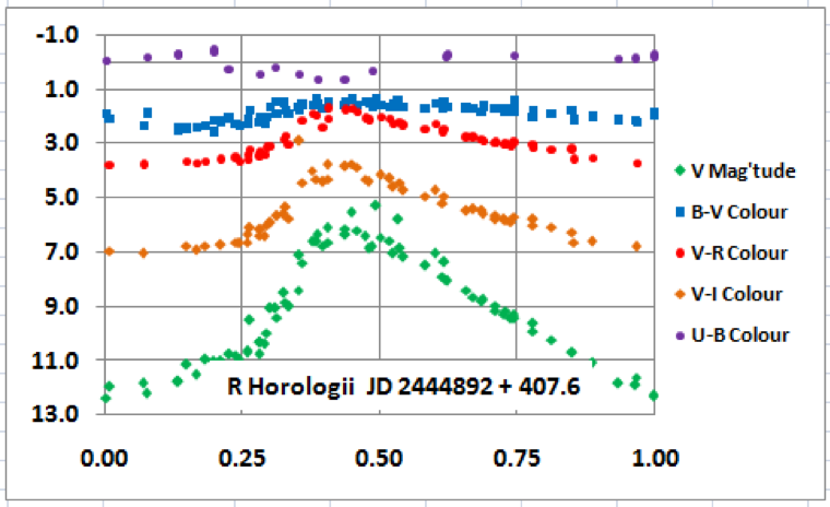
For comparative purposes the visual light curve for 2000 days to July 2018 is presented. The bright maximum just after JD 2456800 is also seen on the phased UBVRI plot, but the visual measures generally show a sharper minimum.

Compatability of Measures:
This brings up the next point - for astrophysical analyses we need an accuracy of ~10 millimagnitudes over decades if the measures are to have value. How do we achieve this? PEP in the southern hemisphere developed differently from that in the north and there were only a small number of participants during the development stages up to about 1980. Even the detectors were different in that most used the expensive but more efficient EMI range of end on photomultiplier tubes. Publication of the Cape Observatory measures in the Royal Observatory Bulletin 64 in 1962 followed by the E and F Region standards allowed everyone to work with stars of reliable magnitudes and colours and this has persisted to the present day.
Johnson and colleagues at Tonantzintla published similar but smaller in number northern UBVRI measures around the same time but later the US Naval Observatory produced a catalogue of many published measures. This illustrated a problem - most stars were listed with a wide range of values - even tau Ceti had values spread over almost half a magnitude. Rather than set up the northern equivalent of the southern sytem using the A and B Harvard regions the sequences were based on clusters which method seems to have its limitations.
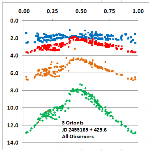
The reaons for the scatter in measures of stars such as S Orionis may be due to poor comparison star values and selection. The sequence for S Orionis lists 22 stars ranging frm V = 7.5 to 14.3, with errors of 0.017 to 0.100 in V and 0.028 to 0.173 in B-V. Mean error values are around 0.050 or more. In the field of R Centauri a query of several stars revealed that some of the values were SPv and SPg, supposedly equivalent to V and B but certainly not so. That system was largely abandoned more than half a century ago.
Let's look at the actual measures of S Orionis to see the problem. Measures from all observers appear on the left, those of Giorgio di Scala on the right. There are some variations in the V light curve as the amplitudes of each cycle are dissimilar. But when plotted as colours these should be much smaller and virtually non-existent in B-V which should only show a smooth, temperature based change. R Horologii above is a good example of compatability over a third of a century and this is the type of result that we need.

Gaia values for many stars have now been released and perhaps the Long Period Variable Section can arrange suitable comparison sequences for LPVs as time permits. It's best to have as few stars as possible and for all observers to be using the same ones as comparisons and checks. How many are needed depends on the range of the Mira in question. The dynamic range of CCDs is much less than pm tubes so the best solution is probably one pair of stars for each 3-4 magnitude interval with the selected stars at mid-range. So for many Miras four stars would be adequate. With most SR stars one pair of stars is enough.
The question of long term variability must also be considered. John Percy in his SARV project concluded that all M type stars are variable to some extent. Whether this is a pulsational variation or merely a result of massive star spots and rotation is not an issue. But it does place a doubt on late K stars, many of which show variations of up to 30 millimags over a decade or two, probably for the same reason. So do we restrict the comparisons to the spectral range A5 to K5? Good transformations will handle the colour differences well.
Spectroscopic Radial Velocity Measures:
Measures of some of the Miras with humps and some of the dual maxima Miras indicate that radius variations may be important in their behaviour. But the radial velocity changes may be small and we are uncertain as to the limits of amateur equipment. If it were possible to make useful measures at this level it would greatly improve our understanding of what is happening during a cycle.
Strange Light Curves:
So far we have discussed fairly normal light curves. But some stars have unusual features in these. Giorgio di Scala's measures of Z Sagittarii are rather unusual in that both B-V and V-R show inversions during about 40% of the cycle and V amplitude variations of two magnitudes. We might attribute the B-V problem to faintness in the B filter but his measures of other stars at B = 18 are quite normal. So the other suspected cause is a blue companion. But it must be an unusual object given the age and brightness of most Miras.


R Carinae is another such object as shown in this illustration of UBV measures from Auckland Observatory in the 1980s. B-V is about 0.7 too bright and U-B at times is slightly negative. Its inversion is due, of course, to an emission shell but here, as perhaps with Z Sagittarii, is a blue or white companion. These may be merely line of sight objects included in the measuring aperture but are more likely to be true companions.
What You Can Do:
Let's put the cart before the horse and convert your measures to V, B-V, U-B, V-I, V-R, R-I and V-I, or any selection of these that you have measured. Since the colour curves should be close to repetitive any large errors will show up. If they do, check your transformations and other things such as extinction corrections.
The AAVSO insists on single filter measures rather than colours but colours are more useful at times in the astrophysical analyses. It helps if you always observe through filters in the same order as it's then quite simple to rearrange them to allow colours to be obtained.
Measures at intervals equal to 5% of the period will define a light curve adequately. Once such a light curve exists it is only necessary to repeat at intervals of a decade unless the star is unusual or very erratic in its behaviour. The best filters are B and V as the historical database is largely made up of such measures.
Monitoring the long term behaviour has largely been the province of visual observers and this will continue to some extent. It's pointless measuring in the V filter only unless someone sets up a systematic programme to measure all the unobserved stars. ASAS3 did this for a time but how complex would it be to set up a programme which measured each of some hundreds of stars in V once each 10 days or so?
For those with the interest, measuring the full BVRI light curves during three or four cycles to build up a graph similat to those shown here has value. Whilst the professional attention has shifted to more statistical surveys each star is different and interesting. The Miras all have an emission shell and often a dust shell as well. So for the former U-B measures, even if they take longer, are valuable during one or two cycles.
The stars with humps look interesting and this is an area which should be explored in more detail. But other unusual Miras such as the dual maxima stars have not been studied in detail and their behaviour is not well understood.
Then there is the whole field of semi-regular stars which because of their mostly low amplitudes are difficult for the visual observers. L2 Puppis has done some interesting things and there are many others of interest. At Auckland we used to look at SY Fornacis as it was once listed as a CV. It is not but it seems to have a blue companion and is listed in different places with three widely separated periods. There are many unstudied SR stars like this.
Little here has been said about JH photometry. In amateur hands it is restricted to the SSP4 photometer which suffers from a number of problems associated with its amplification and detection methods which entail much more time and care per measure. As well, the amplitude range is small at these wavelengths and rather featureless. But it may be that, linked to UBVRI measures at the same phases, it would show something of value. Examples of this are few, if any.